

Wpt (Waypoint) Normalization
By Dr. Max Derhak and Dr. Roy Burns
This article was originally published by the Munsell Color Science Laboratory at RIT.
Introduction
Index
Object-Color Systems
Sensor Adjustment Transforms
von-Kries based SATs
Chromatic Adjustment Transforms
Material Adjustment Transforms
Introducing Wpt
Wpt Normalization Implementation Files (Download)
Useful Wpt Matrices
Object-Color Systems
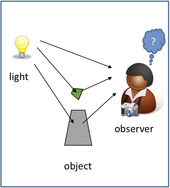
As can be seen in this figure, a simple object-color system is made up of a light source, an object that has a surface that reflects or interacts with light, and an observer or capture system that has sensors/cones that convert light energy into channels of information (hereafter referred to as sensor excitations).
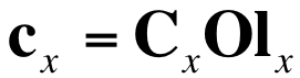
This system is represented for a single object using the following linear (matrix-vector) transformation:
 (1)
(1)
Where:
c defines a vector of resulting sensor excitations,
C defines a matrix containing sensitivity functions, cone fundamentals,
or color-matching functions used to convert incident light to sensor excitations that
may be scaled (normalized) to account for exposure or adjust sensor excitations to a
desired range,
O defines a Donaldson matrix used to define how an object reflects and
emits light at various wavelengths (with spectral reflectance factor defined along the
diagonal),
l defines a vector of the spectral power distribution of the illuminant,
and
x indicates a specific observing condition (i.e., the combination of observer
and illumination).
Sensor Adjustment Transforms
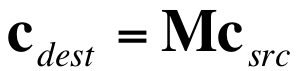
We define a generic linear transform (M) between sensor excitations and adjusted sensor excitations without defining a specific purpose or method as a Sensor Adjustment Transform (SAT), which can be described by the following equation:
 (2)
(2)
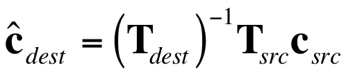
A Sensor Adjustment Transform (SAT) is often used to estimate some form of sensor excitations under one set of observing conditions based upon the sensor excitations under a different set of observing conditions. A SAT utilizes a color equivalency representation or transformation waypoint when such an estimation is made, and the SAT can be decomposed into a sub-transform and an inverse sub-transform. The sub-transforms define the relationships between the sensor excitations and the intermediate color equivalency representation. Thus:
 (3)
(3)
von-Kries based SATs
A von-Kries transform is an example of a transform that utilizes an interim color equivalency representation. A transformation that is mathematically equivalent to a von-Kries transformation is formed by using the following sub-transform definition with the previous equation:
 (4)
(4)
where
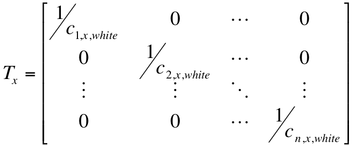
ci,x,white represents the i-th sensor excitation value of white for the observing conditions defined by x.
This sub-transform linearly scales sensor excitations so that white is represented as [1 1 ... 1] with neutrals represented on the line between white and black.
Example 1 - von-Kries illuminant white balancing
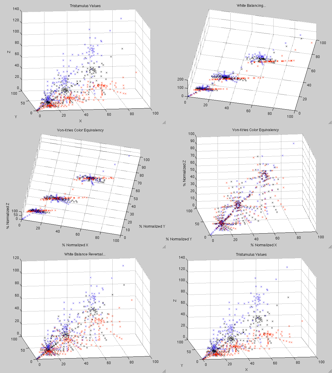
The following animation shows the application and reversal of a von-Kries type sub-transform to sensor excitations (XYZ tristimulus values) of a set of Munsell glossy colors for a standard 2-degree observer under three illuminants (Illuminant A - red, D50 - black, D93 - blue), resulting in a color equivalency representation that has a single representation for white and neutral colors with other colors preserving their linear relationships.
Example 2 - von-Kries observer white balancing
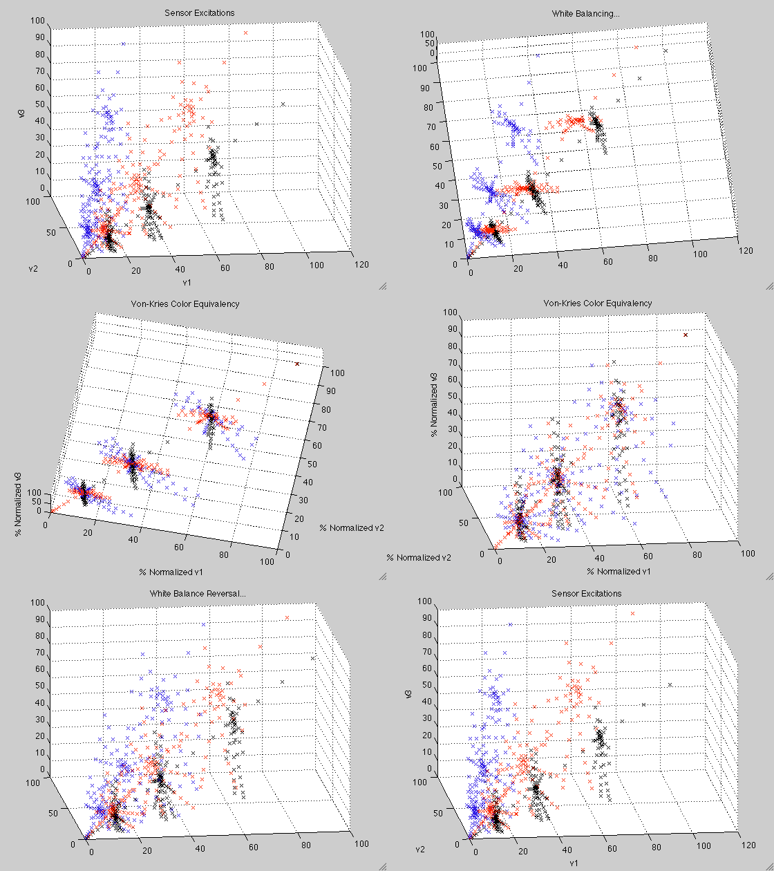
The following animation shows the application and reversal of a von-Kries type sub-transform to sensor excitations (XYZ tristimulus values) of a set of Munsell glossy colors under D65 illumination for three different observers (standard 2-degree - red, CIE 2006 5-degree/45-year-old cone fundamentals - black, CFA digital camera - blue), resulting in a color equivalency representation that has a single representation for white and neutral colors with other colors preserving their linear relationships.
Chromatic Adjustment Transforms (CATs)
One distinct form of a SAT is a Chromatic Adaptation Transform (CAT). A CAT predicts sensor excitations for an observer under one viewing condition that have the same appearance as the observer's sensor excitations under different viewing conditions. Thus, a CAT predicts corresponding color or color appearance. Since corresponding color experiments are based upon judgments of single observers, they provide no information that predicts color appearance between different observers. Therefore, a CAT is inappropriate to use for predicting sensor excitations for one observer based upon sensor excitations of a different observer.
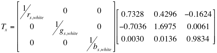
The CAT02 transform is an example of a CAT that first transforms tristimulus (XYZ) values to a sharpened cone space representation before applying a von-Kries type transform to get to a color equivalency representation. Applying the following sub-transform in equation (3) results in a transformation that is mathematically equivalent to the CAT02 transform:
 (5)
(5)
The matrix on the right transforms XYZ values to sharpened cone response values (RGB) in a way that predicts the results of corresponding color experiments. The matrix on the left linearly scales sharpened cone response values so that white is represented as [1 1 1] with neutrals represented on the line between white and black.
Example 3 - CAT02 application
The following animation shows the application and reversal of a CAT02 type sub-transform to sensor excitations (XYZ tristimulus values) of a set of Munsell glossy colors for a standard 2-degree observer under three illuminants (Illuminant A - red, D50 - black, D93 - blue), resulting in a color equivalency representation that estimates corresponding color and has a single representation for white and neutral colors with other colors preserving their linear relationships.
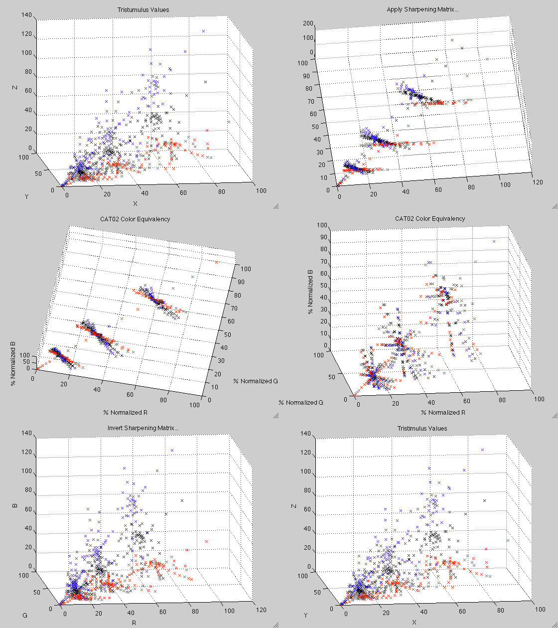
Often partial adaptation is used to represent an incomplete state of adaptation. Partial adaptation is represented by the following adjustment to equation (3):
 (6)
(6)
Material Adjustment Transforms
A distinct form of SAT estimates the sensor excitations of a material object under one set of observing conditions based on the sensor excitations of the same material object under different observing conditions. A SAT that makes such predictions has been designated as a Material Adjustment Transform (MAT) because the material object remains the same. However, the material object may change appearance as a result of the change in observing conditions. This differs from a CAT where the estimation might require a different material object to preserve color appearance.
A MAT utilizes an intermediate color equivalency representation that preserves or estimates material color, and therefore, it is appropriate to use a MAT for relating sensor excitations of colors for changes in illuminant and/or observer. The color equivalency representation utilized by MATs is generally related to a set of reference objects for a reference observer under a reference illuminant. Therefore, any difference between actual sensor excitations and estimated sensor excitations represents a material color shift due to illuminant and/or observer metamerism of the objects involved.
Introducing Wpt (pronounced Waypoint)
A normalization methodology has been developed that linearly transforms sensor excitations (or linear transforms of sensor excitations) into a material color equivalency representation that can be used as a waypoint for defining Material Adjustment Transforms. The normalization process adjusts for the white point and independently preserves the perceptive aspects of lightness, chroma, and hue, resulting in an opponent-like coordinate system designated by the axes W, p, and t.
Wpt normalization is performed by applying a sequence of linear transforms to observer- and illuminant-specific sensor excitations for reference colors that are concatenated into a single linear transformation matrix (A). The general sequence of transforms is as follows:
- The sensor excitations for white (a perfect reflecting diffuser) are rotated to align with the first axis (W).
- The first axis is scaled so that white has a value of (100, 0, 0).
- A plane is first fitted to a set of chromatic colors with constant chroma and constant lightness, and then the coefficients of the plane are used to shear sensor excitations so that a set of reference colors with constant lightness fall on a plane that is orthogonal to the first axis.
- Regression is used to determine a linear transform that minimizes differences in hue and chroma for a set of reference colors that have constant chroma and lightness.
Note: For the reference observing conditions, step 4 is replaced with an iterative application of fitting sensor excitations for a set of reference colors that have constant chroma and lightness with an equation for an ellipse, and then using rotation and scaling so they are approximately constant in distance from the first W (achromatic axis), with vivid yellow falling on the positive t axis and red colors having positive p (second axis) values. The resulting p and t values for this set of reference colors are then used for regression purposes in step 4 for non-reference conditions.
Example 4 - Wpt normalization for different illuminants
The following animation shows the application and reversal of Wpt normalization steps to sensor excitations (XYZ tristimulus values) of a set of Munsell glossy colors for a standard 2-degree observer under three illuminants (Illuminant A - red, D50 - black, D93 - blue).
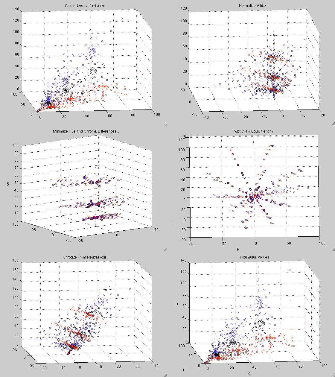
Example 5 - Wpt normalization for different observers
The following animation shows the application and reversal of Wpt normalization steps to sensor excitations (XYZ tristimulus values) of a set of Munsell glossy colors under a D65 illuminant for three different observers (standard 2-degree - red, CIE 2006 5-degree/45-year-old cone fundamentals - black, CFA digital camera - blue).
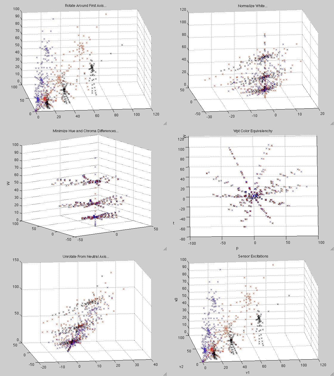
Observations about Wpt normalization
There are three key features that make Wpt unique and advantageous as a color space:
- Differences due to changes in illuminant or observer are minimized as part of the Wpt normalization process. Thus, Wpt provides a singular material color equivalency representation that is appropriate for defining Material Adjustment Transforms.
- Wpt normalization using different observers that satisfy the same Luther-Ives conditions results in different normalization matrices that transform sensor excitations to identical Wpt coordinates. Thus, Wpt coordinates are unique for an observer independent of whether color matching functions or cone fundamentals are used.
- Wpt preserves the linear relationships of sensor excitations and the polar form of Wpt preserves the perceptive aspects of lightness, chroma, and hue. Therefore, Wpt normalization adjustments for differences in observing conditions are always represented as positive lightness, chroma, and hue even though the corresponding sensor excitations may have negative values.
However, Wpt is not perceptually uniform and therefore constant differences in Wpt coordinates do not represent constant perceptual differences. For a perceptually uniform space based upon Wpt, use WLab.
Wpt implementation files
The following zip file contains MATLAB/Octave code that can be used to perform Wpt
normalization. The files dumpWptMATs.m and plotWpts.m can
be used as references for creating and using structures containing Wpt normalization
matrices.
The following Excel file can be used to determine a Wpt normalization matrix specific to an observer and illuminant.
Useful Wpt Matrices
The following is the resulting output from the dumpWptMATs MATLAB/Octave
function in the above zip archive. These matrices may be useful when implementation of
Wpt normalization is not needed. It is assumed that each matrix will be applied to a
column vector containing XYZ tristimulus values.
Wpt Normalization Matrices
| 2-deg/D65 XYZ to Wpt | ||
|---|---|---|
| 0.02964 | 0.97487 | -0.00280 |
| 4.83916 | -4.73122 | 0.12117 |
| 0.54248 | 1.30671 | -1.67368 |
| 2-deg/D50 XYZ to Wpt | ||
|---|---|---|
| -0.06265 | 1.03839 | 0.02669 |
| 4.68561 | -4.82563 | 0.37293 |
| 0.28350 | 1.50053 | -2.15101 |
| 2-deg/Illum A XYZ to Wpt | ||
|---|---|---|
| -0.33810 | 1.30006 | 0.20048 |
| 4.40232 | -5.32134 | 1.36425 |
| -0.41103 | 2.17849 | -4.85343 |
| 2-deg/Illum C XYZ to Wpt | ||
|---|---|---|
| -0.00000 | 1.00000 | -0.00000 |
| 4.84591 | -4.80280 | 0.04258 |
| 0.51873 | 1.30963 | -1.53805 |
| 2-deg/Illum E XYZ to Wpt | ||
|---|---|---|
| -0.07407 | 1.05436 | 0.01971 |
| 4.61340 | -4.78331 | 0.16986 |
| 0.37630 | 1.40421 | -1.78050 |
| 2-deg/F11 XYZ to Wpt | ||
|---|---|---|
| -0.12366 | 1.05659 | 0.10608 |
| 4.38611 | -4.63611 | 0.32299 |
| 0.37476 | 1.29098 | -2.59413 |
| 10-deg/D65 XYZ to Wpt | ||
|---|---|---|
| 0.07837 | 0.99300 | -0.06271 |
| 5.12107 | -5.27209 | 0.38828 |
| 0.78225 | 1.13989 | -1.75315 |
| 10-deg/D50 XYZ to Wpt | ||
|---|---|---|
| -0.03390 | 1.06622 | -0.04107 |
| 4.98326 | -5.37826 | 0.68588 |
| 0.48282 | 1.35138 | -2.23437 |
| 10-deg/Illum A XYZ to Wpt | ||
|---|---|---|
| -0.36233 | 1.37188 | 0.08758 |
| 4.76102 | -5.94588 | 1.85883 |
| -0.29792 | 2.07286 | -4.94818 |
| 10-deg/Illum C XYZ to Wpt | ||
|---|---|---|
| 0.04888 | 1.02268 | -0.06047 |
| 5.14072 | -5.36078 | 0.30964 |
| 0.75497 | 1.15250 | -1.62468 |
| 10-deg/Illum E XYZ to Wpt | ||
|---|---|---|
| -0.04091 | 1.08336 | -0.04246 |
| 4.89821 | -5.31600 | 0.41832 |
| 0.59264 | 1.24324 | -1.83564 |
| 10-deg/F11 XYZ to Wpt | ||
|---|---|---|
| -0.13853 | 1.11178 | 0.04893 |
| 4.73751 | -5.27217 | 0.53588 |
| 0.47386 | 1.20030 | -2.57966 |
Wpt based MATs
| 10-deg/D65 XYZ to 2-deg/D65 XYZ | ||
|---|---|---|
| 1.10560 | -0.09275 | -0.00471 |
| 0.04656 | 1.02167 | -0.06132 |
| -0.07267 | 0.08653 | 0.99808 |
| 2-deg/D65 XYZ to 2-deg/D50 XYZ | ||
|---|---|---|
| 1.13639 | -0.05000 | -0.06045 |
| 0.09798 | 0.93483 | -0.02568 |
| -0.03407 | 0.03805 | 0.75221 |
| 10-deg/D65 XYZ to 10-deg/A XYZ | ||
|---|---|---|
| 1.74309 | -0.34150 | -0.18609 |
| 0.52037 | 0.63017 | -0.11512 |
| -0.04504 | 0.05418 | 0.31728 |